Finding least-squares solutions
Prerequisites
We’ll assume you that you have read this post on least-squares solution and the normal equation
Finding least-squares solutions
In this post, we’ll see the numpy code for doing linear regression by solving the normal equation \(X^TX\theta = X^TY\).
If there are \(n\) data points and \(k\) features for each data point, then \(X\) is an \(n\times (k+1)\) matrix. Further if \(X\) has zero kernel, then there is a unique solution to the normal equation given by
\[\theta = (X^TX)^{-1}X^TY\]Finding \(\theta\) in this manner would typically involve inverting \(X^TX\) which is an \((k+1)\times (k+1)\) matrix. Inverting matrices is an expensive operation (the complexity of this inversion would be around \(O(k^3)\)), so ML packages use other methods to do linear regression like gradient descent etc. Nevertheless, it’s useful to know how to solve the normal equation, so we persevere ahead.
Imports
As before, we’ll be using libraries like pandas, numpy, matplotlib and scikit-learn. So you’ll have to preface your code with the following import statements.
#Imports
import pandas as pd
import matplotlib.pyplot as plt
plt.style.use('classic')
import numpy as np

from sklearn.model_selection import train_test_split
from sklearn.metrics import mean_squared_error
The weather dataset yet again
Let’s continue with our weather example from before. Say we have access to the average daily temperature \(T\), the wind-gut \(W\) , and the total minutes of sunshine \(S\) per day. These will be our features. We would like to predict the amount of precipitation \(P\) each day using linear regression.
Code:
col_names = ['date','avgtemp', 'mintemp', 'pp', 'snow', 'wind-dir', 'wind-speed', 'wind-gut', 'air-pressure', 'sunshine', 'dummy']

#Reads the comma separated csv into a pandas dataframe
daily_weather_df =pd.read_csv('KCQT0.csv', sep=',',names=col_names, header = None)

#Delete irrelevant cols
del daily_weather_df['dummy']
del daily_weather_df['air-pressure']
del daily_weather_df['wind-speed']
del daily_weather_df['snow']
del daily_weather_df['wind-dir']
del daily_weather_df['date']
del daily_weather_df['mintemp']

#Delete rows with NaN entries
daily_weather_df.dropna(inplace=True)

#Drop precipitation column to get weather_features
weather_features = daily_weather_df.drop(['pp'], axis=1)
precipitation_targets = daily_weather_df['pp']


print(weather_features.head())
print(precipitation_targets.head())
Features:
| avgtemp | wind-gut | sunshine | |
|---|---|---|---|
| 0 | 10.4 | 2.0 | 1018.9 |
| 1 | 12.0 | 8.1 | 1021.0 |
| 2 | 11.4 | 1.3 | 1026.5 |
| 3 | 12.6 | 3.0 | 1024.9 |
| 4 | 13.3 | 1.9 | 1018.0 |
Target:
0    13.9
1    15.6
2    18.9
3    20.0
4    21.7
Name: pp, dtype: float64
We are trying to find a linear relationship between \(P, T, W, S\). That is, we’d like to find \(\theta_0, \theta_1, \theta_2, \theta_3\) so that
\[P = \theta_0 + \theta_1 T + \theta_2 W + \theta_3 S\]Splitting into training and test data sets
Code:
#Declare random state to be an int to get reproducible output, shuffle is True by default
X_train, X_test, y_train, y_test = train_test_split(weather_features, precipitation_targets,
                                                    test_size=0.30, random_state=10, shuffle=True)

print(f"Training data : {X_train.shape}, {y_train.shape}")
print(f"Test data : {X_test.shape}, {y_test.shape}")
Output:
Training data : (1306, 3), (1306,)
Test data : (560, 3), (560,)
Massaging the training data into the right type and shape
Let’s understand the types of our training and test data
print(f"Training data type : {type(X_train)}, {type(y_train)}")
print(f"Test data type : {type(X_test)}, {type(y_test)}")
Training data type : <class 'pandas.core.frame.DataFrame'>, <class 'pandas.core.series.Series'>
Test data type : <class 'pandas.core.frame.DataFrame'>, <class 'pandas.core.series.Series'>
Ah, they are Pandas dataframes. Let’s convert them to numpy arrays to make it easier to work with, with respect to the task of solving the normal equation.
X_train_numpy = X_train.to_numpy()
print(type(X_train_numpy), X_train_numpy.shape)
print(X_train_numpy)
<class 'numpy.ndarray'> (1306, 3)
[[  19.4    4.8 1013. ]
 [  18.3    2.  1017.6]
 [  12.5    1.6 1024. ]
 ...
 [  19.9    4.4 1014.7]
 [  14.7    4.2 1014.4]
 [  19.9    3.4 1007.7]]
Remember, we have to add the dummy feature \(x_i^0=1\) to each data point.
training_data_points = X_train_numpy.shape[0]
#Concatenate the dummy 0th feature x_i^0 = 1 for each training data point
X = np.c_[np.ones((training_data_points,1)), X_train_numpy]
print(f"Shape of X is {X.shape}")
print(X)
Shape of X is (1306, 4)
[[1.0000e+00 1.9400e+01 4.8000e+00 1.0130e+03]
 [1.0000e+00 1.8300e+01 2.0000e+00 1.0176e+03]
 [1.0000e+00 1.2500e+01 1.6000e+00 1.0240e+03]
 ...
 [1.0000e+00 1.9900e+01 4.4000e+00 1.0147e+03]
 [1.0000e+00 1.4700e+01 4.2000e+00 1.0144e+03]
 [1.0000e+00 1.9900e+01 3.4000e+00 1.0077e+03]]
Let’s also convert the target variable values in the training dataset to a numpy array
Y=y_train.to_numpy()
print(type(Y), Y.shape)
<class 'numpy.ndarray'> (1306,)
Solving the normal equation
The numpy code to find transposes, inverses, take dot products or multiply matrices is easy. In particular, \(X.T\) is the transpose of \(X\), \(np.linalg.inv(X)\) is \(X^{-1}\) and \(a.dot(b)\) is the dot-product of \(a\) and \(b\).
Let’s convert the formula \(\theta = (X^TX)^{-1}X^TY\) into python code now.
theta_best = np.linalg.inv(X.T.dot(X)).dot(X.T).dot(Y)
print(f" Shape of theta_best is {theta_best.shape}")
print(f" theta_best is {theta_best}")
 Shape of theta_best is (4,)
 theta_best is [-1.89711155e+02  1.28170996e+00 -3.04886864e-01  1.88450340e-01]
Predictions
Let’s now massage the test data into the right type and shape also!
X_test_numpy = X_test.to_numpy()
test_data_points = X_test_numpy.shape[0]
#Concatenate the dummy 0th feature x_i^0 = 1 for each test data point
X_test_numpy = np.c_[np.ones((test_data_points,1)), X_test_numpy]
y_test_numpy = y_test.to_numpy()
Let’s look at how to predict the target variable for a single test data point.
#Getting a single test data point
y_test_singleton = y_test_numpy[0]
#Prediction for a single test data point
y_pred_singleton = X_test_numpy[0].dot(theta_best)
print(f"The true value : {y_test_singleton}")
print(f"The predicted value : {y_pred_singleton}")
The true value : 20.6
The predicted value : 22.874195641340407
Let’s now predict the target variable for the entire test data set.
#Predictions for the test data set
y_pred = X_test_numpy.dot(theta_best)
print(f"Shape of y_test_numpy is {y_test_numpy.shape}")
print(f"Shape of y_pred is {y_pred.shape}")
Shape of y_test_numpy is (560,)
Shape of y_pred is (560,)
Evaluation of predictions
#Root mean squared error between predictions and test values
print(f"Root mean squared error : {mean_squared_error(y_test_numpy,y_pred,squared=False)}")
Root mean squared error : 1.5578231355991063
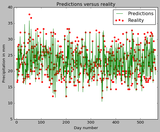
Like before, we also draw a simple plot of reality versus the predictions.
evaluation_of_predictions=plt.figure()
plt.scatter(range(1,561),y_test_numpy, color="red", label="Reality");
plt.plot(range(1,561),y_predict, color="green",label="Predictions");
plt.xlim(-10,570)
plt.title("Predictions versus reality")
plt.xlabel("Day number")
plt.ylabel("Precipitation in mm");
plt.legend();
Comparison to earlier validation-error estimate
The root mean squared error on our test-data set from our decision tree regressor on the same dataset earlier was around 1.77. We see that the root mean squared error has gone down to 1.56 for our linear regressor.